Convolutional neural network
Convolutional Neural Network
Primarily used for image tasks such as computer vision or image generation, though they can be used anywhere you have a rectangular grid with spatial relationship among your data.
Typically convolutional layers are used in blocks consisting of the following:
- Conv2D layer.
- Usually stride 2 for encoders, stride 1 for decoders.
- Often includes some type of padding such as zero padding.
- Upscale layer (for decoders only).
- Normalization or pooling layer (e.g. Batch normalization or Max Pool).
- Activation (typically ReLU or some variant).
More traditionally, convolutional blocks came in blocks of two conv layers
- Conv2D layer.
- Activation.
- Conv2d Layer.
- Activation.
- Max pool or Avg pool
Upsampling blocks also have a transposed convolution or a bilinear upsample in the beginning.
The last layer is typically just a \(\displaystyle 1 \times 1\) or \(\displaystyle 3 \times 3\) Conv2D with a possible sigmoid to control the range of the outputs.
Motivation
Convolutional neural networks leverage the following properties of images:
- Stationarity or shift-invariance - objects in an image should be recognized regardless of their position
- Locality or local-connectivity - nearby pixels are more relevant than distant pixels
- Compositionality - objects in images have a multi-resolution structure.
Convolutions
Pytorch Convolution Layers
Types of convolutions animations
Here, we will explain 2d convolutions, also known as cross-correlation.
Suppose we have the following input image:
1 2 3 4 5
6 7 8 2 3
2 5 9 9 5
4 8 8 2 1
and the following 3x3 kernel:
1 1 1
2 1 2
3 2 1
For each possible position of the 3x3 kernel over the input image,
we perform an element-wise multiplication (\(\displaystyle \odot\)) and sum over all entries to get a single value.
Placing the kernel in the first position would yield:
\(\displaystyle
\begin{bmatrix}
1 & 2 & 3\\
6 & 7 & 8\\
2 & 5 & 9
\end{bmatrix}
\odot
\begin{bmatrix}
1 & 1 & 1\\
2 & 1 & 2\\
3 & 2 & 1
\end{bmatrix}
=
\begin{bmatrix}
1 & 2 & 3\\
12 & 7 & 16\\
6 & 10 & 9
\end{bmatrix}
\)
Summing up all the elements gives us \(\displaystyle 66\) which would go in the first index of the output.
Shifting the kernel over all positions of the image gives us the whole output, another 2D image.
The formula for the output resolution of a convolution is: \(\displaystyle \frac{x-k+2p}{s}+1 \) where:
- \(x\) is the input resolution
- \(k\) is the kernel size (e.g. 3)
- \(p\) is the padding on each side
- \(s\) is the stride
Typically a \(3 \times 3\) conv layer will have a padding of 1 and stride of 1 to maintain the same size. A stride of \(2\) would halve the resolution.
Kernel
Typically these days people use small kernels e.g. \(3 \times 3\) or \(4 \times 4\) with many conv layers.
However, historically people used larger kernels (e.g. \(\displaystyle 7 \times 7\)). This leads to more parameters which need to be trained and thus networks cannot be as deep.
Note that in practice, people use multi-channel inputs so the actual kernel will be 3D.
A Conv2D layer with \(C_1\) input channels and \(C_2\) output channels will have \(C_2\) number of \(3 \times 3 \times C_1\) kernels.
However, we still call this Conv2D because the kernel moves in 2D only.
Similarly, a Conv3D layer will typically have multiple 4D kernels.
Stride
How much the kernel moves. Typically 1 or 2.
Moving by 2 will yield half the resolution of the input.
Padding
Convolutional layers typically yield an output smaller than the input size.
We can use padding to increase the input size.
See Machinecurve: Using Constant Padding, Reflection Padding and Replication Padding with Keras
- Common Types of padding
- Zero or Constant padding
- Mirror/Reflection padding
- Replication padding
With convolution layers in libraries you often see these two types of padding which can be added to the conv layer directly:
VALID- Do not do any paddingSAME- Apply zero padding such that the output will have resolution \(\lfloor x/stride \rfloor\).- \(p=\frac{k-1}{2}\)
- Exact behavior varies between ML frameworks. Only apply this when you know you will have symmetric padding on both sides.
Dilation
Space between pixels in the kernel
A dilation of 1 will apply a 3x3 kernel over a 5x5 region. This would be equivalent to a 5x5 kernel with odd index weights (\(\displaystyle i \% 2 == 1\)) set to 0.
- These are used in Atrous Spatial Pyramid Pooling (ASPP), where different dilation amounts mimic a UNet's spatial pyramid.
- The pro is that ASPP uses less computation since there are fewer kernels (i.e. fewer channels). The con is that it takes up more memory.
Groups
Other Types of Convolutions
Transpose Convolution
See Medium: Transposed convolutions explained.
Instead of your 3x3 kernel taking 9 values as input and returning 1 value: \(\sum_i \sum_j w_{ij} * i_{i+x,j+y}\), the kernel now takes 1 value and returns 9 values: \(w_{ij} * i_{x,y}\).
This is sometimes misleadingly referred to as deconvolution.
Oftentimes, papers apply a 2x bilinear upsampling rather than using transpose convolution layers.
Gated Convolution
See Gated Convolution (ICCV 2019)
Given an image, we have two convolution layers \(\displaystyle k_{feature}\) and \(\displaystyle k_{gate}\).
The output is \(\displaystyle O = \phi(k_{feature}(I)) \odot \sigma(k_{gate}(I))\)
Pooling

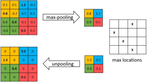
Pooling is one method of reducing and increasing the resolution of your feature maps.
You can also use bilinear upsampling or downsampling.
Typically the stride of pooling is equal to the filter size so a \(\displaystyle 2 \times 2\) pooling will have a stride of \(\displaystyle 2\) and result in an image with half the width and height.
Avg Pooling
Take the average over a region.
This is equivalent to bilinear downsampling.
Max Pooling
Take the max over a region.
Unpooling
During max pooling, remember the indices where you pulled from in switch variables.
Then when unpooling, save the max value into those indices. Other indices get values of 0.
Spherical Images
There are many ways to adapt convolutional layers to spherical images.
- Learning Spherical Convolution for Fast Features from 360 Imagery (NIPS 2017) proposes using different kernels with different weights and sizes for different altitudes \(\phi\).
- Circular Convolutional Neural Networks (IV 2019) proposes padding the left and right sides of each input and feature map using pixels such that the input wraps around. This works since equirectangular images wrap around on the x-axis.
- SpherePHD (CVPR 2019) proposes using faces of an icosahedron as pixels. They propose a kernel which considers the neighboring 9 triangles of each triangle. They also develop methods for pooling.
- CoordConv (NeurIPS 2018) adds additional channels to each 2D convolution layer which feeds positional information (UV coordinates) to the convolutional kernel. This allows the kernel to account for distortions. Note that the positional information is merely UV coordinates and is not learned like in NLP.
- Jiang et al. (ICLR 2019) perform convolutions on meshes using linear combination of first order derivatives and the Laplacian second order derivative. These derivatives are estimated based on the values and positions of neighboring vertices and faces. Experiments are performed on a sphere mesh.
