360SD-Net: 360° Stereo Depth Estimation with Learnable Cost Volume

360SD-Net: 360° Stereo Depth Estimation with Learnable Cost Volume (ICRA 2020)

Published in 2020 IEEE International Conference on Robotics and Automation (ICRA 2020)

Authors: Ning-Hsu Wang, Bolivar Solarte1, Yi-Hsuan Tsai, Wei-Chen Chiu, Min Sun
Affiliations: National Tsing Hua University, NEC Labs America, National Chiao Tung University

• Arxiv Mirror ntcu.edu.tw paper mirror
• Project Page GitHub
• Dataset Request Form

Architecture

Architecture Figure from their paper

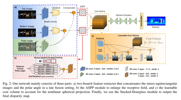
Their input is two equirectangular images, one taken above another.
They also input the polar angle:

# Y angle
angle_y = np.array([(i-0.5)/512*180 for i in range(256, -256, -1)])
angle_ys = np.tile(angle_y[:, np.newaxis, np.newaxis], (1,1024, 1))
equi_info = angle_ys

The angles are equivalent to np.linspace(90, -90, height+1)[:-1] - 0.5*(180/height) and broadcast into an \([H, W, 1]\) image tensor.

Feature Extraction

They first feed both input images individually into a CNN with and a resblock.
They also feed the polar angle image into a separate CNN.
Then they concatenate the features for the polar angle images into the features for each input image separately.

The resblock in their image is actually 3+16+3+3=25 blocks.
Each block contains: conv-batchnorm-relu-conv-batchnorm.
The input to each block is elementwise added to the output.
The output number of channels of each block is:

# Each basic block is conv-batchnorm-relu-conv-batchnorm with a residual connection.
# self._make_layer(block, channels, num_blocks, stride, pad, dilation) 
# makes a sequential network with `num_blocks` number of `block`
# each of which outputs `channels` number of channels.

self.layer1 = self._make_layer(BasicBlock, 32, 3, 1,1,1)
self.layer2 = self._make_layer(BasicBlock, 64, 16, 2,1,1) 
self.layer3 = self._make_layer(BasicBlock, 128, 3, 1,1,1)
self.layer4 = self._make_layer(BasicBlock, 128, 3, 1,1,2)

My Questions

• The polar angle image is the same for all images.
  • How is this different from just concatenating a variable and optimizing that variable independently?

ASPP Module

Atrous-Spatial Pyramid Pooling

This idea comes from Chen et al..

The idea here is to perform convolution over multiple scales of the input image or feature tensor.
This is performed using multiple parallel convolutions of the input, each with different dilation sizes.

#... make model
def convbn(in_planes, out_planes, kernel_size, stride, pad, dilation):
    return nn.Sequential(
        nn.Conv2d(in_planes,
                  out_planes,
                  kernel_size=kernel_size,
                  stride=stride,
                  padding=dilation if dilation > 1 else pad,
                  dilation=dilation,
                  bias=False), nn.BatchNorm2d(out_planes))


self.aspp1 = nn.Sequential(convbn(160, 32, 1, 1, 0, 1), nn.ReLU(inplace=True))
self.aspp2 = nn.Sequential(convbn(160, 32, 3, 1, 1, 6), nn.ReLU(inplace=True))
self.aspp3 = nn.Sequential(convbn(160, 32, 3, 1, 1, 12), nn.ReLU(inplace=True))
self.aspp4 = nn.Sequential(convbn(160, 32, 3, 1, 1, 18), nn.ReLU(inplace=True))
self.aspp5 = nn.Sequential(convbn(160, 32, 3, 1, 1, 24), nn.ReLU(inplace=True))

#... call
ASPP1 = self.aspp1(output_skip_c)
ASPP2 = self.aspp2(output_skip_c)
ASPP3 = self.aspp3(output_skip_c)
ASPP4 = self.aspp4(output_skip_c)
ASPP5 = self.aspp5(output_skip_c)
output_feature = torch.cat((output_raw, ASPP1,ASPP2,ASPP3,ASPP4,ASPP5), 1)

Learnable Cost Volume

A disparity space image (DSI) is a 2D tensor which stores the matching values between two scanlines.
In 3D (with 2D images rather than 1D scanlines), it is called a 3D cost volume.
Each slice \(i\) is computed by taking images \(I_1\) and \(I_2\), sliding image \(I_2\) down by \(i\) pixels, and subtracting them to yield

# This is not their actual code. Their actual code is slightly more complicated.
cost_volume[:,:,i] = I_1 - stack(tile(I_2[:1,:], [i,1]), I_2[i:,:], axis=0)

They learn the optimal step sizes by applying a 7x1 Conv2D CNN.

Their cost volume code

cost = Variable(torch.FloatTensor(refimg_fea.size()[0], refimg_fea.size()[1]*2, self.maxdisp/4 *3,  refimg_fea.size()[2],  refimg_fea.size()[3]).zero_()).cuda()

for i in range(self.maxdisp/4 *3):
    if i > 0 :
        cost[:, :refimg_fea.size()[1], i, :,:]   = refimg_fea[:,:,:,:]
        cost[:, refimg_fea.size()[1]:, i, :,:] = shift_down[:,:,:,:]
        shift_down = self.forF(shift_down)
    else:
        cost[:, :refimg_fea.size()[1], i, :,:]   = refimg_fea
        cost[:, refimg_fea.size()[1]:, i, :,:]   = targetimg_fea
        shift_down = self.forF(targetimg_fea)

cost = cost.contiguous()

3D Encoder-Decoder

Next they pass the cost volume into a 3 3D hourglass encoder-decoder CNNs which regress the stereo disparity.

They use an l1 loss against the ground truth disparity, which they can get from the depth.

Dataset

They construct a dataset using Matterport3D and Stanford 3D datasets. Their constructed dataset is available upon request.