Image Registration

Image registration is recovering an affine transformation (rotation + translation) between two images.

Image registration can be performed in the frequency domain with the Fourier transform or in the spatial domain with a log-polar transformation.

Problem Statement

We are given two images \(\displaystyle I_1\) and \(\displaystyle I_2\).
Let \(\displaystyle (x,y)\) be uv coordinates within the image.
We want to find a rotation and translation from \(\displaystyle (x,y)\) to \(\displaystyle (x',y')\) such that \(\displaystyle I_1(x,y) = I_2(x', y')\).
This is represented as:
\( \begin{align} x' &= a_1 x + a_2 y + a_3\\ y' &= a_4 x + a_5 y + a_6 \end{align} \)
This can also be written as:
\(\displaystyle \begin{pmatrix} x' \\ y' \\ 1 \end{pmatrix} = \begin{pmatrix} a_1 & a_2 & a_3\\ a_4 & a_5 & a_6\\ 0 & 0 & 1 \end{pmatrix} \begin{pmatrix} x \\ y \\ 1 \end{pmatrix} \)

Log-Polar Transformation

This is copied from Wolberg and Zokai.

The log-polar transformation is defined as follows:
\( \begin{align} \rho &= \log(r) = \log\left(\sqrt{(x-x_c)^2 + (y-y_c)^2}\right)\\ \theta &= \operatorname{arctan2}(y-y_c, x-x_c) \end{align} \)
where \(\displaystyle (x_c, y_c)\) is the center of the image and \(\displaystyle r\) is the distance from the center of the image.

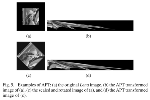
Here a rotation in Cartesian coordinates \(\displaystyle (x, y)\) around the center \((x_c, y_c)\) corresponds to a shift in \(\theta\) in log-polar coordinates.

A scale change (i.e. enlarge or stretch) is a shift in log-space:
\( \lambda r \mapsto \log(\lambda r) = \log(\lambda) + \log(r) \)

These translations can be found using Wikipedia: Cross-correlation.

Algorithm

For each resolution from coarse to fine, do the following:

1. Crop central region \(\displaystyle I_1'\) from \(\displaystyle I_1\)
2. Compute the low-polar transformation \(\displaystyle I_{1p}'\)
3. For all positions \((x,y)\)
   1. Crop region \(I_{2p}'\)
   2. Compute \(I_{2p}'\)
   3. Cross-correlate \(I_{1p}'\) and \(I_{2p}'\) to get \((dx, dy)\)
   4. If max correlation, save \((x, y)\) and \((dx, dy)\)
4. Scale = \(dx\)
5. Rotation = \(dy\)
6. Translation = \(x, y\)

Adaptive Log-Polar Transformation

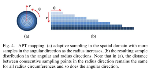
The goal of Adaptive Polar Transform by Matungka et al. is to address the non-uniform sampling of the log-polar transformation.

Motivation

Let the following:

• \(n_\rho\) be the number of samples (i.e. resolution) along the \(\rho\) axis
• \(n_\theta\) be the number of samples along the \(\theta\) axis
• \(r_i\) the radius size for pixel \(i=1,...,n_\rho\)
• \(\theta = 0,...,n_\theta - 1\)

To prevent undersampling along \(\rho\), we must have \(R_{n_\rho} - R_{n_\rho-1} \leq 1\). I.e. the outermost two circles must have \(\leq 1\) pixel difference.
To prevent undersampling along \(\theta\), we must have at least \(2\pi R_{max}\) pixels along the \(\theta\) axis.

This leads to the following equations:
\[ \begin{align} R_i &= \exp(i \times \frac{\log R_{max}}{n_\rho}), \qquad R_{max} = R_{n_\rho}\\ n_\rho &\geq \frac{\log R_{max}}{\log R_{max} - \log(R_{max}-1)}\\ n_\theta &\geq 2\pi R_{max} \end{align} \]

However, using these would lead to oversampling of the fovea region wasting computation resources.

Let the following:

• \(n_r\) be the number of samples (i.e. resolution) along the \(r\) axis
• \(n_\theta\) be the number of samples along the \(\theta\) axis

Given an image of size \(2 R_{max} \times 2 R_{max}\), let (R_i\) the radius size for pixel \(i=1,...,n_\rho\).

The main idea is that the number of pixels \(n_\theta\) should be adaptive to the radius: \[ \begin{align} n_r &= R_{max}\\ n_{\theta_i} &= R_i \end{align} \]

To transform an image \(I\) to adaptive polar \(IP\), do the following

for i=1 to n_r
  for j=1 to n_{theta_i}
    IP(i,j)=I(R_max + R_i*cos(2*pi*j/n_theta_i),
              R_max + R_i*sin(2*pi*j/n_theta_i))

The paper continues to define a projection \(\mathfrak{R}, \Theta\) to a 1-d image: \[ \Theta(j) = \sum_{i=1}^{n_4}\left[ \eta_{ij}^1 IP\left(i, \left\lceil\frac{j-1}{\Omega_i}\right\rceil\right) + \eta^2_{ij}IP\left(i, \left\lceil\frac{j}{\Omega_i}\right\rceil\right) \right] \] where:

• \(i \in [1,...,n_r]\)
• \(j \in [1,...,\hat{n}_\theta\)
• \(\Omega_i = \frac{\hat{n}_0}{n_{\theta_i}}\)
• \(\eta_{ij}^1=\Omega_i(j-1) - \lfloor \Omega_i(j-1)\rfloor\)
• \(\eta_{ij}^2=1-\eta_{ij}^1\)
• \(IP(i, 0) = 0 \quad \forall i\)

Then:

• A scale change appears as variable-scale i.e. \(\mathbfrak{R_1(\lambda r)\) while \(\Theta\) is slightly altered.
• A rotation in the cartesian image appears as a phase-shift in \(\Theta\).

References

- ↑ George Wolberg, and Siavash Zokai (2000). Robust Image Registration Using Log-Polar Transform DOI: 10.1109/ICIP.2000.901003 URL: https://home.cis.rit.edu/~cnspci/references/wolberg2000.pdf
- ↑ Rittavee Matungka, Yuan F. Zheng, and Robert L. Ewing (2009). Image Registration Using Adaptive Polar Transform DOI: 10.1109/TIP.2009.2025010 URL: https://home.cis.rit.edu/~cnspci/references/wolberg2000.pdf