Image Registration: Difference between revisions
Created page with "Image registration is recovering an affine transformation (rotation + translation) between two images." |
|||
| (25 intermediate revisions by the same user not shown) | |||
| Line 1: | Line 1: | ||
Image registration is recovering an affine transformation (rotation | Image registration is recovering an affine transformation (scale, rotation, translation) between two images. | ||
Image registration can be performed in the frequency domain with the Fourier transform or in the spatial domain with a log-polar transformation. | |||
==Problem Statement== | |||
We are given two images <math>I_1</math> and <math>I_2</math>.<br> | |||
Let <math>(x,y)</math> be uv coordinates within the image.<br> | |||
We want to find a rotation and translation from <math>(x,y)</math> to <math>(x',y')</math> such that <math>I_1(x,y) = I_2(x', y')</math>.<br> | |||
This is represented as:<br> | |||
\( | |||
\begin{align} | |||
x' &= a_1 x + a_2 y + a_3\\ | |||
y' &= a_4 x + a_5 y + a_6 | |||
\end{align} | |||
\)<br> | |||
This can also be written as:<br> | |||
<math> | |||
\begin{pmatrix} | |||
x' \\ y' \\ 1 | |||
\end{pmatrix} | |||
= | |||
\begin{pmatrix} | |||
a_1 & a_2 & a_3\\ | |||
a_4 & a_5 & a_6\\ | |||
0 & 0 & 1 | |||
\end{pmatrix} | |||
\begin{pmatrix} | |||
x \\ y \\ 1 | |||
\end{pmatrix} | |||
</math> | |||
==Phase correlation== | |||
{{main | Wikipedia: Phase correlation}} | |||
By the [https://en.wikipedia.org/wiki/Discrete_Fourier_transform#Shift_theorem Fourier shift theorem], a translation in the spatial domain is a linear phase shift in the Fourier domain.<br> | |||
Hence, if you have two images with only a translation, you can identify the translation by estimating the phase shift. | |||
==Log-Polar Transformation== | |||
This is copied from Wolberg and Zokai<ref name="wolberg2000robust"/>. See also Reddy (1996)<ref name="reddy1996fft"/>. | |||
The log-polar transformation is defined as follows:<br> | |||
\( | |||
\begin{align} | |||
\rho &= \log(r) = \log\left(\sqrt{(x-x_c)^2 + (y-y_c)^2}\right)\\ | |||
\theta &= \operatorname{arctan2}(y-y_c, x-x_c) | |||
\end{align} | |||
\)<br> | |||
where <math>(x_c, y_c)</math> is the center of the image and <math>r</math> is the distance from the center of the image. | |||
Here a rotation in Cartesian coordinates <math>(x, y)</math> around the center \((x_c, y_c)\) corresponds to a shift in \(\theta\) in log-polar coordinates. | |||
A scale change (i.e. enlarge or stretch) is a shift in log-space:<br> | |||
\( \lambda r \mapsto \log(\lambda r) = \log(\lambda) + \log(r) \)<br> | |||
These translations can be found using [[Wikipedia: Cross-correlation]] or [[Wikipedia: Phase correlation]]. | |||
;Algorithm | |||
For each resolution from coarse to fine, do the following: | |||
# Crop central region <math>I_1'</math> from <math>I_1</math> | |||
# Compute the low-polar transformation <math>I_{1p}'</math> | |||
# For all positions \((x,y)\) | |||
## Crop region \(I_{2p}'\) | |||
## Compute \(I_{2p}'\) | |||
## Cross-correlate \(I_{1p}'\) and \(I_{2p}'\) to get \((dx, dy)\) | |||
## If max correlation, save \((x, y)\) and \((dx, dy)\) | |||
# Scale = \(dx\) | |||
# Rotation = \(dy\) | |||
# Translation = \(x, y\) | |||
===Adaptive Log-Polar Transformation=== | |||
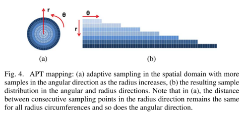
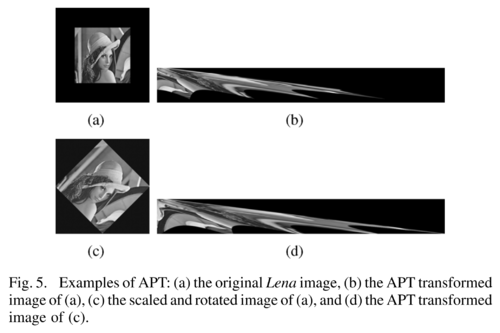
The goal of Adaptive Polar Transform by Matungka ''et al.''<ref name="matungka2009adaptive"/> is to address the non-uniform sampling of the log-polar transformation. | |||
[[File: Adaptive polar transform fig4.png | 500px | Adaptive Polar Transform]] | |||
[[File: Adaptive polar transform fig5.png | 500px | Adaptive Polar Transform Lena]] | |||
{{ hidden | Motivation | | |||
Let the following: | |||
* \(n_\rho\) be the number of samples (i.e. resolution) along the \(\rho\) axis | |||
* \(n_\theta\) be the number of samples along the \(\theta\) axis | |||
* \(r_i\) the radius size for pixel <math display="inline">i=1,...,n_\rho</math> | |||
* <math display="inline">\theta = 0,...,n_\theta - 1</math> | |||
To prevent undersampling along \(\rho\), we must have \(R_{n_\rho} - R_{n_\rho-1} \leq 1\). | |||
I.e. the outermost two circles must have \(\leq 1\) pixel difference.<br> | |||
To prevent undersampling along \(\theta\), we must have at least \(2\pi R_{max}\) pixels along the \(\theta\) axis. | |||
This leads to the following equations:<br> | |||
<math display="block"> | |||
\begin{align} | |||
R_i &= \exp(i \times \frac{\log R_{max}}{n_\rho}), \qquad R_{max} = R_{n_\rho}\\ | |||
n_\rho &\geq \frac{\log R_{max}}{\log R_{max} - \log(R_{max}-1)}\\ | |||
n_\theta &\geq 2\pi R_{max} | |||
\end{align} | |||
</math> | |||
However, using these would lead to oversampling of the fovea region wasting computation resources. | |||
}} | |||
Let the following: | |||
* \(n_r\) be the number of samples (i.e. resolution) along the \(r\) axis | |||
* \(n_\theta\) be the number of samples along the \(\theta\) axis | |||
Given an image of size \(2 R_{max} \times 2 R_{max}\), let (R_i\) the radius size for pixel \(i=1,...,n_\rho\). | |||
The main idea is that the number of pixels \(n_\theta\) should be adaptive to the radius: | |||
\[ | |||
\begin{align} | |||
n_r &= R_{max}\\ | |||
n_{\theta_i} &= R_i | |||
\end{align} | |||
\] | |||
To transform an image \(I\) to adaptive polar \(IP\), do the following | |||
<pre> | |||
for i=1 to n_r | |||
for j=1 to n_{theta_i} | |||
IP(i,j)=I(R_max + R_i*cos(2*pi*j/n_theta_i), | |||
R_max + R_i*sin(2*pi*j/n_theta_i)) | |||
</pre> | |||
The paper continues to define a projection \(\mathfrak{R}, \Theta\) to a 1-d image: | |||
\[ | |||
\Theta(j) = \sum_{i=1}^{n_4}\left[ \eta_{ij}^1 IP\left(i, \left\lceil\frac{j-1}{\Omega_i}\right\rceil\right) + \eta^2_{ij}IP\left(i, \left\lceil\frac{j}{\Omega_i}\right\rceil\right) \right] | |||
\] | |||
where: | |||
* \(i \in [1,...,n_r]\) | |||
* \(j \in [1,...,\hat{n}_\theta\) | |||
* \(\Omega_i = \frac{\hat{n}_0}{n_{\theta_i}}\) | |||
* \(\eta_{ij}^1=\Omega_i(j-1) - \lfloor \Omega_i(j-1)\rfloor\) | |||
* \(\eta_{ij}^2=1-\eta_{ij}^1\) | |||
* \(IP(i, 0) = 0 \quad \forall i\) | |||
Then: | |||
* A scale change appears as ''variable-scale'' i.e. \(\mathfrak{R}_1(\lambda r)\) while \(\Theta\) is slightly altered. | |||
* A rotation in the cartesian image appears as a phase-shift in \(\Theta\).<br> | |||
==References== | |||
{{reflist|refs= | |||
<ref name="wolberg2000robust">George Wolberg, and Siavash Zokai (2000). ''Robust Image Registration Using Log-Polar Transform'' DOI: [https://doi.org/10.1109/ICIP.2000.901003 10.1109/ICIP.2000.901003] URL: [https://home.cis.rit.edu/~cnspci/references/wolberg2000.pdf https://home.cis.rit.edu/~cnspci/references/wolberg2000.pdf]</ref> | |||
<ref name="reddy1996fft">B. S. Reddy and B. N. Chatterji, "An FFT-based technique for translation, rotation, and scale-invariant image registration," in IEEE Transactions on Image Processing, vol. 5, no. 8, pp. 1266-1271, Aug. 1996, doi: 10.1109/83.506761. https://ieeexplore.ieee.org/document/506761</ref> | |||
<ref name="matungka2009adaptive"><cite class="journal">Rittavee Matungka, Yuan F. Zheng, and Robert L. Ewing (2009). ''Image Registration Using Adaptive Polar Transform'' DOI: [https://doi.org/10.1109/TIP.2009.2025010 10.1109/TIP.2009.2025010] URL: [https://home.cis.rit.edu/~cnspci/references/wolberg2000.pdf https://home.cis.rit.edu/~cnspci/references/wolberg2000.pdf]</cite></ref> | |||
}} | |||
Latest revision as of 17:28, 28 June 2023
Image registration is recovering an affine transformation (scale, rotation, translation) between two images.
Image registration can be performed in the frequency domain with the Fourier transform or in the spatial domain with a log-polar transformation.
Problem Statement
We are given two images \(\displaystyle I_1\) and \(\displaystyle I_2\).
Let \(\displaystyle (x,y)\) be uv coordinates within the image.
We want to find a rotation and translation from \(\displaystyle (x,y)\) to \(\displaystyle (x',y')\) such that \(\displaystyle I_1(x,y) = I_2(x', y')\).
This is represented as:
\(
\begin{align}
x' &= a_1 x + a_2 y + a_3\\
y' &= a_4 x + a_5 y + a_6
\end{align}
\)
This can also be written as:
\(\displaystyle
\begin{pmatrix}
x' \\ y' \\ 1
\end{pmatrix}
=
\begin{pmatrix}
a_1 & a_2 & a_3\\
a_4 & a_5 & a_6\\
0 & 0 & 1
\end{pmatrix}
\begin{pmatrix}
x \\ y \\ 1
\end{pmatrix}
\)
Phase correlation
By the Fourier shift theorem, a translation in the spatial domain is a linear phase shift in the Fourier domain.
Hence, if you have two images with only a translation, you can identify the translation by estimating the phase shift.
Log-Polar Transformation
This is copied from Wolberg and Zokai[1]. See also Reddy (1996)[2].
The log-polar transformation is defined as follows:
\(
\begin{align}
\rho &= \log(r) = \log\left(\sqrt{(x-x_c)^2 + (y-y_c)^2}\right)\\
\theta &= \operatorname{arctan2}(y-y_c, x-x_c)
\end{align}
\)
where \(\displaystyle (x_c, y_c)\) is the center of the image and \(\displaystyle r\) is the distance from the center of the image.
Here a rotation in Cartesian coordinates \(\displaystyle (x, y)\) around the center \((x_c, y_c)\) corresponds to a shift in \(\theta\) in log-polar coordinates.
A scale change (i.e. enlarge or stretch) is a shift in log-space:
\( \lambda r \mapsto \log(\lambda r) = \log(\lambda) + \log(r) \)
These translations can be found using Wikipedia: Cross-correlation or Wikipedia: Phase correlation.
- Algorithm
For each resolution from coarse to fine, do the following:
- Crop central region \(\displaystyle I_1'\) from \(\displaystyle I_1\)
- Compute the low-polar transformation \(\displaystyle I_{1p}'\)
- For all positions \((x,y)\)
- Crop region \(I_{2p}'\)
- Compute \(I_{2p}'\)
- Cross-correlate \(I_{1p}'\) and \(I_{2p}'\) to get \((dx, dy)\)
- If max correlation, save \((x, y)\) and \((dx, dy)\)
- Scale = \(dx\)
- Rotation = \(dy\)
- Translation = \(x, y\)
Adaptive Log-Polar Transformation
The goal of Adaptive Polar Transform by Matungka et al.[3] is to address the non-uniform sampling of the log-polar transformation.
Let the following:
- \(n_\rho\) be the number of samples (i.e. resolution) along the \(\rho\) axis
- \(n_\theta\) be the number of samples along the \(\theta\) axis
- \(r_i\) the radius size for pixel \(i=1,...,n_\rho\)
- \(\theta = 0,...,n_\theta - 1\)
To prevent undersampling along \(\rho\), we must have \(R_{n_\rho} - R_{n_\rho-1} \leq 1\).
I.e. the outermost two circles must have \(\leq 1\) pixel difference.
To prevent undersampling along \(\theta\), we must have at least \(2\pi R_{max}\) pixels along the \(\theta\) axis.
This leads to the following equations:
\[
\begin{align}
R_i &= \exp(i \times \frac{\log R_{max}}{n_\rho}), \qquad R_{max} = R_{n_\rho}\\
n_\rho &\geq \frac{\log R_{max}}{\log R_{max} - \log(R_{max}-1)}\\
n_\theta &\geq 2\pi R_{max}
\end{align}
\]
However, using these would lead to oversampling of the fovea region wasting computation resources.
Let the following:
- \(n_r\) be the number of samples (i.e. resolution) along the \(r\) axis
- \(n_\theta\) be the number of samples along the \(\theta\) axis
Given an image of size \(2 R_{max} \times 2 R_{max}\), let (R_i\) the radius size for pixel \(i=1,...,n_\rho\).
The main idea is that the number of pixels \(n_\theta\) should be adaptive to the radius: \[ \begin{align} n_r &= R_{max}\\ n_{\theta_i} &= R_i \end{align} \]
To transform an image \(I\) to adaptive polar \(IP\), do the following
for i=1 to n_r
  for j=1 to n_{theta_i}
    IP(i,j)=I(R_max + R_i*cos(2*pi*j/n_theta_i),
              R_max + R_i*sin(2*pi*j/n_theta_i))
The paper continues to define a projection \(\mathfrak{R}, \Theta\) to a 1-d image: \[ \Theta(j) = \sum_{i=1}^{n_4}\left[ \eta_{ij}^1 IP\left(i, \left\lceil\frac{j-1}{\Omega_i}\right\rceil\right) + \eta^2_{ij}IP\left(i, \left\lceil\frac{j}{\Omega_i}\right\rceil\right) \right] \] where:
- \(i \in [1,...,n_r]\)
- \(j \in [1,...,\hat{n}_\theta\)
- \(\Omega_i = \frac{\hat{n}_0}{n_{\theta_i}}\)
- \(\eta_{ij}^1=\Omega_i(j-1) - \lfloor \Omega_i(j-1)\rfloor\)
- \(\eta_{ij}^2=1-\eta_{ij}^1\)
- \(IP(i, 0) = 0 \quad \forall i\)
Then:
- A scale change appears as variable-scale i.e. \(\mathfrak{R}_1(\lambda r)\) while \(\Theta\) is slightly altered.
- A rotation in the cartesian image appears as a phase-shift in \(\Theta\).
References
<templatestyles src="Reflist/styles.css" />
- ↑ George Wolberg, and Siavash Zokai (2000). Robust Image Registration Using Log-Polar Transform DOI: 10.1109/ICIP.2000.901003 URL: https://home.cis.rit.edu/~cnspci/references/wolberg2000.pdf
- ↑ B. S. Reddy and B. N. Chatterji, "An FFT-based technique for translation, rotation, and scale-invariant image registration," in IEEE Transactions on Image Processing, vol. 5, no. 8, pp. 1266-1271, Aug. 1996, doi: 10.1109/83.506761. https://ieeexplore.ieee.org/document/506761
- ↑ Rittavee Matungka, Yuan F. Zheng, and Robert L. Ewing (2009). Image Registration Using Adaptive Polar Transform DOI: 10.1109/TIP.2009.2025010 URL: https://home.cis.rit.edu/~cnspci/references/wolberg2000.pdf


